Plotting#

Functions for plotting the input data, inference results, and convergence/stability metrics.

`proxy_strat`	Plot stratigraphic data (proxy observations and age constraints) for each section.
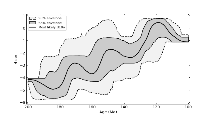
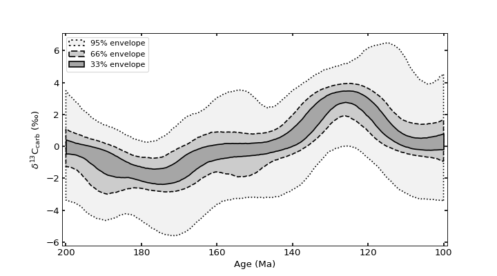
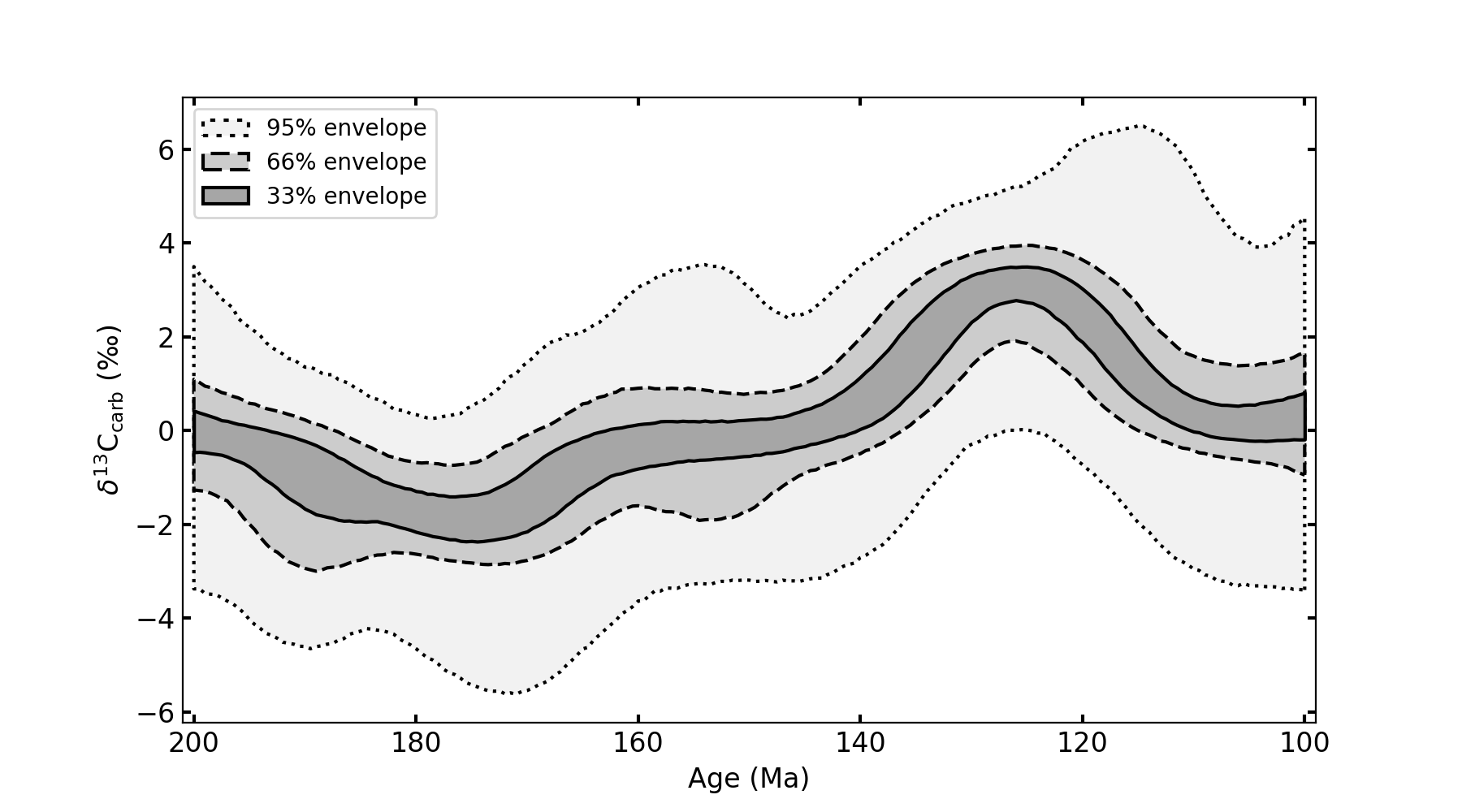
`proxy_inference`	Plot the inferred proxy signal over time.
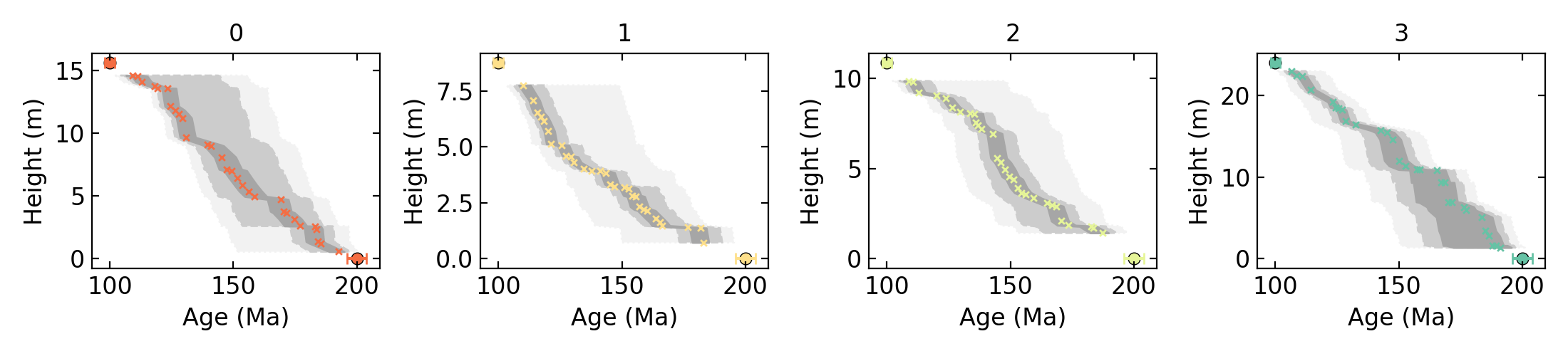
`interpolated_proxy_inference`	Plot interpolated proxy signal over time (by extending the posterior section age models to a new proxy not included in the inference model) using interpolated age models from `extend_age_model()` and interpolated proxy values from `interpolate_proxy()` in `stratmc.inference`.
`age_height_model`	Generate a posterior age-height plot for each section.
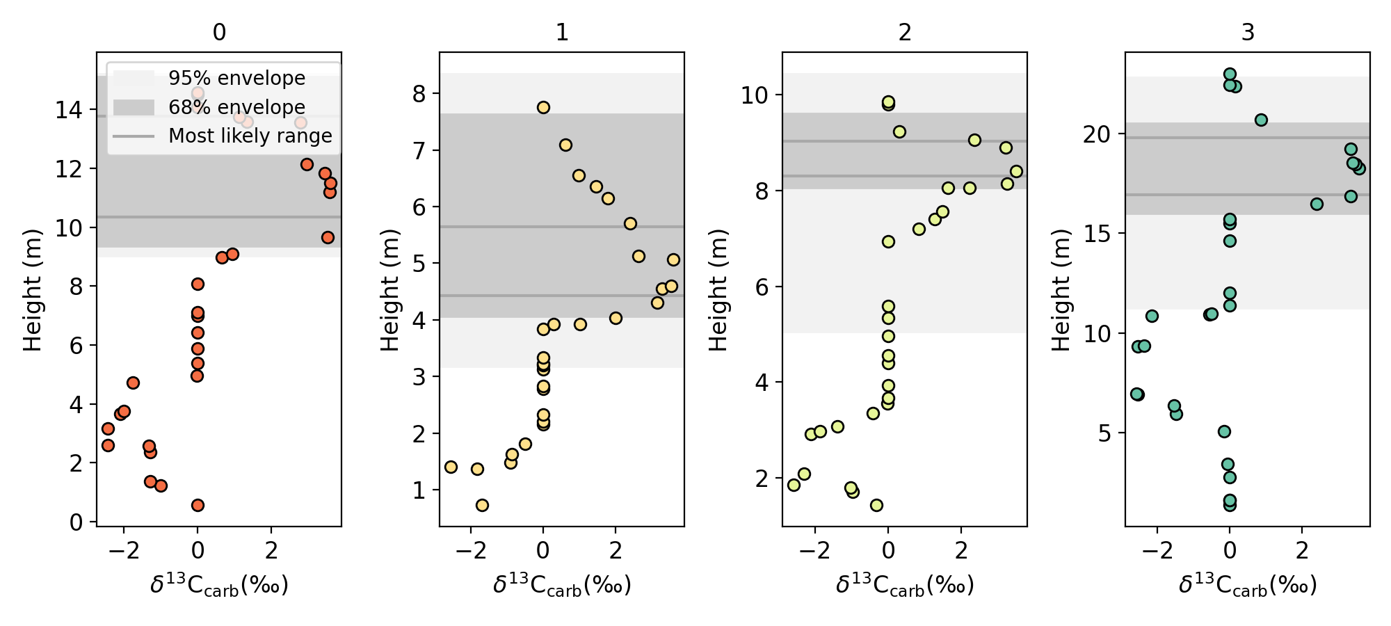
`section_proxy_signal`	Map the posterior proxy signal back to height in each section (using its most likely posterior age model), and plot alongside the proxy observations (plotted by most likely posterior age).
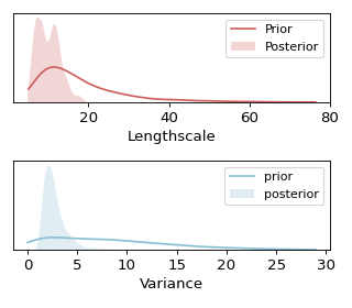
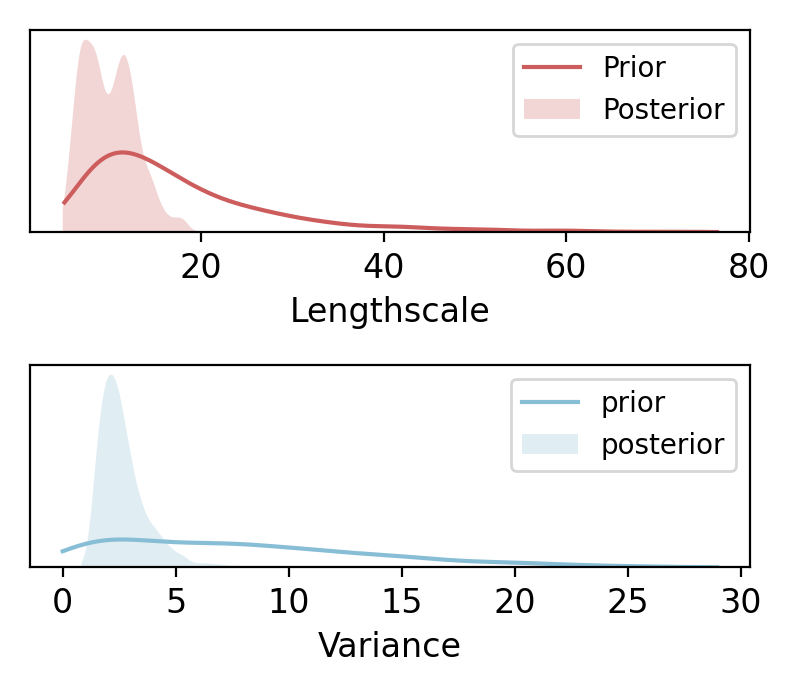
`covariance_hyperparameters`	Plot prior and posterior distributions for the lengthscale (\(\ell\)) and variance (\(\sigma\)) hyperparameters of the `pymc.gp.cov.ExpQuad` Gaussian process covariance kernel:
`section_summary`	For a given section, plot posterior estimates of sample age, sedimentation rate, noise, and offset.
`noise_summary`	Plot posterior noise distributions for each section or group of samples (depending on `noise_type` used in `build_model()`) for a given proxy.
`offset_summary`	Plot posterior offset distributions for each section or group of samples (depending on `offset_type` used in `build_model()`).
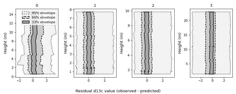
`section_proxy_residuals`	Plot the residuals between the observed proxy values for each section and the inferred proxy signal (using the posterior section age models to map the signal back to height in section).
`sample_ages`	Plot sample age prior and posterior distributions for a given section.
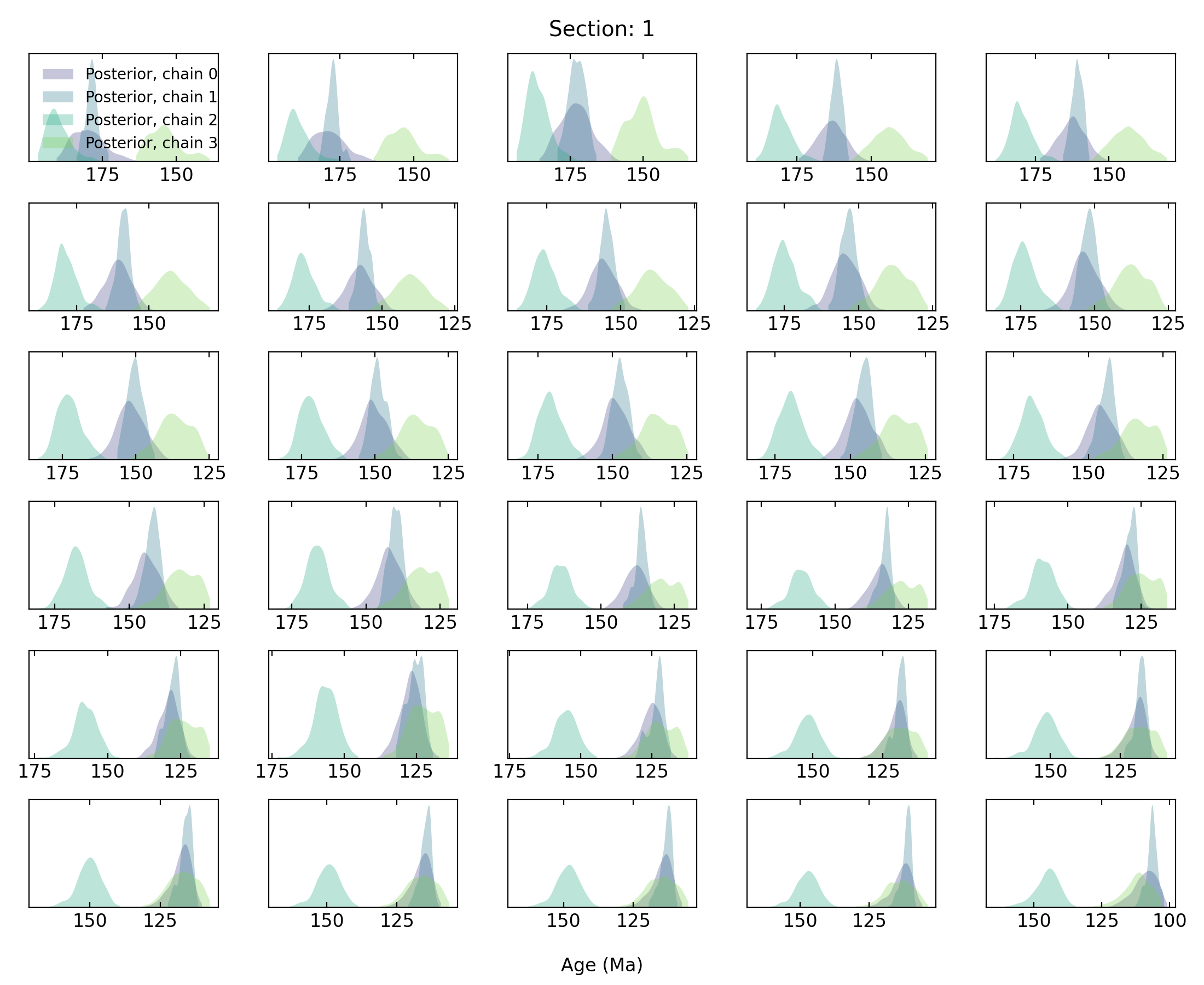
`sample_ages_per_chain`	Plot sample age posterior distributions for a given section, with separate distributions for each chain.
`age_constraints`	For a given section, plot prior and posterior age distributions for all depositional age constraints (and limiting age constraints that provide a minimum or maximum age for the entire section).
`limiting_age_constraints`	For a given section, plot prior and posterior age distributions for all intermediate limiting (i.e., detrital and intrusive ages in the middle of a section) age constraints.
`sadler_plot`	Plot accumulation rate against duration.
`accumulation_rate_stratigraphy`	Plot the probability density of sediment accumulation rates (calculated between successive samples) through time.
`section_age_range`	Plot the stratigraphic interval corresponding to a given age range (based on the posterior section age models).
`proxy_data_gaps`	For a set of discrete time bins, shows the number of draws from the posterior where there are no proxy observations (i.e., where there are temporal gaps in the proxy data).
`proxy_data_density`	Plot the mean number proxy observations in discrete time bins (averaged over all posterior draws).
`lengthscale_traceplot`	Generate trace plot (parameter value vs.
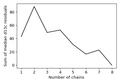
`lengthscale_stability`	Plot the posterior standard deviation of the `pymc.gp.cov.ExpQuad` covariance kernel lengthscale when 1 through N chains are considered.
`proxy_signal_stability`	Plot the sum (over all time slices) of the residuals between the median inferred proxy signal when all N chains are considered compared to when 1 to N-1 chains are considered.

stratmc.plotting.accumulation_rate_stratigraphy(full_trace, sample_df, ages_df, age_bins=50, age_bin_edges=[], rate_bins=50, rate_bin_edges=[], rate_scale='log', include_age_constraints=True, cmap='jet', figsize=(8, 4), **kwargs)[source]#

Plot the probability density of sediment accumulation rates (calculated between successive samples) through time. Probability density for each age bin sums to 1. Unless a sections argument is passed, includes accumulation rates for all sections.

(Source code, png, hires.png, pdf)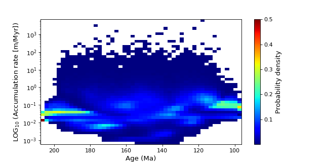

Parameters:

full_trace: arviz.InferenceData: An arviz.InferenceData object containing the full set of prior and posterior samples from get_trace() in stratmc.inference.
sample_df: pandas.DataFrame: pandas.DataFrame containing proxy data for all sections.
ages_df: pandas.DataFrame: pandas.DataFrame containing age constraints for all sections.
age_bins: int, optional: Number of bin edges for age data (if age_bin_edges not provided). Defaults to 50.
rate_bins: int, optional: Number of bin edges for rate data (if rate_bin_edges not provided). Defaults to 50.
age_bin_edges: list(float) or numpy.array(float), optional: List or array of bin edges for the age data.
rate_bin_edges: list(float) numpy.array(float), optional: List or array of bin edges for the rate data.
rate_scale: str, optional: Scaling for rate (‘linear’ or ‘log’). Defaults to ‘log’.
include_age_constraints: bool, optional: Include age constraints in sedimentation rate calculations. Defaults to True.
sections: list(str) or numpy.array(str), optional: Section(s) to include. If not provided, combines data from all sections in sample_df.

Returns:

fig: matplotlib.pyplot.figure: Figure with accumulation rate probability density through time.

stratmc.plotting.age_constraints(full_trace, section, cmap='viridis', **kwargs)[source]#

For a given section, plot prior and posterior age distributions for all depositional age constraints (and limiting age constraints that provide a minimum or maximum age for the entire section). To plot intermediate limiting ages (i.e., detrital and intrusive age constraints in the middle of a section), use limiting_age_constraints().

(Source code, png, hires.png, pdf)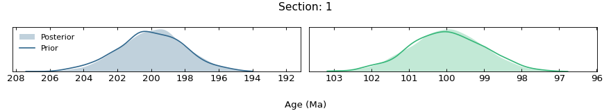

Parameters:

full_trace: arviz.InferenceData: An arviz.InferenceData object containing the full set of prior and posterior samples from get_trace() in stratmc.inference.
section: str: Name of target section.
cmap: str, optional: Name of seaborn color palette to use for age distributions. Defaults to ‘viridis’.

Returns:

fig: matplotlib.pyplot.figure: Figure with prior and posterior depositional age constraint distributions.

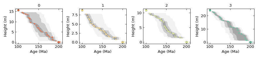
stratmc.plotting.age_height_model(sample_df, ages_df, full_trace, include_excluded_samples=True, plot_samples=True, cmap='Spectral', legend=False, **kwargs)[source]#

Generate a posterior age-height plot for each section.

(Source code, png, hires.png, pdf)

Parameters:

sample_df: pandas.DataFrame: pandas.DataFrame containing proxy data for all sections.
ages_df: pandas.DataFrame: pandas.DataFrame containing age constraints for all sections.
full_trace: arviz.InferenceData: An arviz.InferenceData object containing the full set of prior and posterior samples from get_trace() in stratmc.inference.
sections: list(str) or numpy.array(str), optional: List of sections to plot. Defaults to all sections in sample_df.
cmap: str, optional: Name of seaborn color palette to use for sections. Defaults to ‘Spectral’.
legend: bool, optional: Generate a legend. Defaults to False.
include_excluded_samples: bool, optional: Whether to consider excluded samples (Exclude? is True in sample_df) whose ages were passively tracked in the inference model. Defaults to True.
plot_samples: bool, optional: Plot proxy observations by most likely posterior age. Defaults to True.

Returns:

fig: matplotlib.pyplot.figure: Figure with age-height models for each section.

stratmc.plotting.covariance_hyperparameters(full_trace, figsize=(4, 3.5), **kwargs)[source]#

Plot prior and posterior distributions for the lengthscale (\(\ell\)) and variance (\(\sigma\)) hyperparameters of the pymc.gp.cov.ExpQuad Gaussian process covariance kernel:

\[k(x, x') = \sigma^2 \mathrm{exp} \left[-\frac{(x - x')^2}{2 \ell^2} \right]\]

(Source code, png, hires.png, pdf)

Parameters:

full_trace: arviz.InferenceData: An arviz.InferenceData object containing the full set of prior and posterior samples from get_trace() in stratmc.inference.
proxy: str, optional: Tracer to plot model parameters for (each proxy has a different covariance kernel); only required if more than one proxy was included in the inference.

Returns:

fig: matplotlib.pyplot.figure: Figure with prior and posterior model parameters.

stratmc.plotting.interpolated_proxy_inference(interpolated_df, interpolated_proxy_df, proxy, legend=True, plot_samples=False, plot_mle=True, orientation='horizontal', section_legend=False, marker_size=20, section_cmap='Spectral', **kwargs)[source]#

Plot interpolated proxy signal over time (by extending the posterior section age models to a new proxy not included in the inference model) using interpolated age models from extend_age_model() and interpolated proxy values from interpolate_proxy() in stratmc.inference.

(Source code, png, hires.png, pdf)

Parameters:

interpolated_df: pandas.DataFrame: pandas.DataFrame with interpolated age draws and sample age summary statistics from extend_age_model() in stratmc.inference.
interpolated_proxy_df: pandas.DataFrame: pandas.DataFrame with interpolated proxy values and summary statistics at target ages from interpolate_proxy() in stratmc.inference.
proxy: str: Name of new proxy (must match column name in interpolated_proxy_df).
legend: bool, optional: Generate a legend. Defaults to True.
plot_samples: bool, optional: Plot proxy observations by most likely posterior age. Defaults to False.
plot_mle: bool, optional: Plot the maximum likelihood estimate. Defaults to True.
orientation: str, optional: Orientation of figure (‘horizontal’ or ‘vertical’). Defaults to ‘horizontal’.
marker_size: int, optional: Size of markers if plot_samples is True. Defaults to 20.
section_legend: bool, optional: Include section names in the legend (if plot_samples is True). Defaults to False.
section_cmap: str, optional: Name of seaborn color palette to use for sections (if plot_samples is True). Defaults to ‘Spectral’.

Returns:

fig: matplotlib.pyplot.figure: Figure with interpolated proxy signal over time.

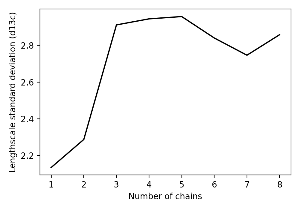
stratmc.plotting.lengthscale_stability(full_trace, figsize=(5, 3.5), **kwargs)[source]#

Plot the posterior standard deviation of the pymc.gp.cov.ExpQuad covariance kernel lengthscale when 1 through N chains are considered. When the posterior has been sufficiently explored, the standard deviation will stabilize; if it has not stabilized, then additional chains should be run.

To consider chains from multiple traces associated with the same inference model, first combine the traces (saved as NetCDF files) using combine_traces() in stratmc.data.

(Source code, png, hires.png, pdf)

Parameters:

full_trace: arviz.InferenceData: An arviz.InferenceData object containing the full set of prior and posterior samples from get_trace() in stratmc.inference.
proxy: str, optional: Target proxy; only required if more than one proxy was included in the inference.

Returns:

fig: matplotlib.pyplot.figure: Figure showing the standard deviation of the covariance kernel lengthscale hyperparameter posterior for 1 through N chains.

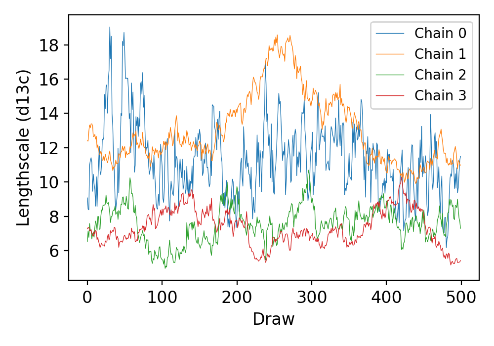
stratmc.plotting.lengthscale_traceplot(full_trace, chains=None, legend=True, figsize=(5, 3.5), **kwargs)[source]#

Generate trace plot (parameter value vs. step in Markov chain) for the pymc.gp.cov.ExpQuad covariance kernel lengthscale. By default, includes all chains; to plot the draws for only a subset of chains, past list of chain indices to chains. Use to check for posterior multimodality.

(Source code, png, hires.png, pdf)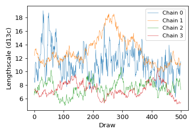

Parameters:

full_trace: arviz.InferenceData: An arviz.InferenceData object containing the full set of prior and posterior samples from get_trace() in stratmc.inference.
chains: list(int) or numpy.array(int); optional: Indices of chains to plot; optional (defaults to all chains).
proxy: str, optional: Target proxy; only required if more than one proxy was included in the inference.
legend: bool, optional: Generate a legend. Defaults to True.

Returns:

fig: matplotlib.pyplot.figure: Figure with lengthscale trace plot.

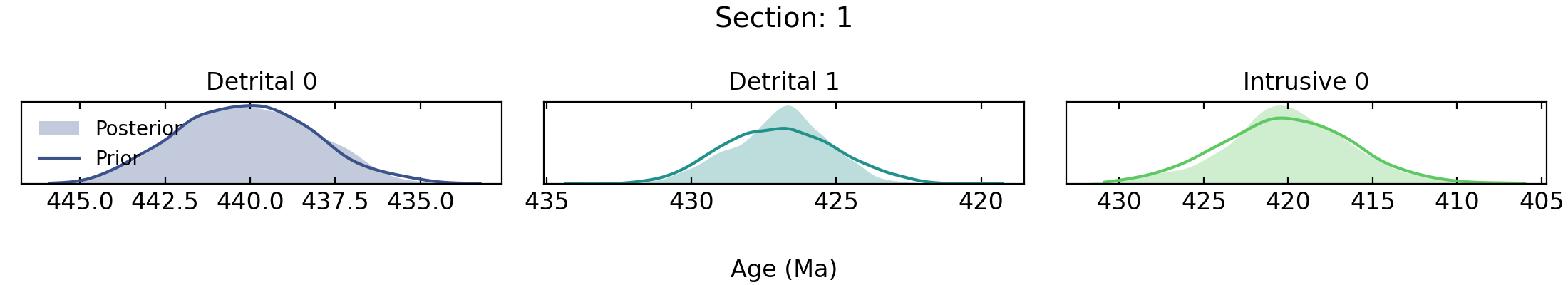
stratmc.plotting.limiting_age_constraints(full_trace, sample_df, ages_df, section, cmap='viridis', **kwargs)[source]#

For a given section, plot prior and posterior age distributions for all intermediate limiting (i.e., detrital and intrusive ages in the middle of a section) age constraints. To plot depositional age constraints (and limiting age constraints that provide a minimum or maximum age for the entire section), use age_constraints().

(Source code, png, hires.png, pdf)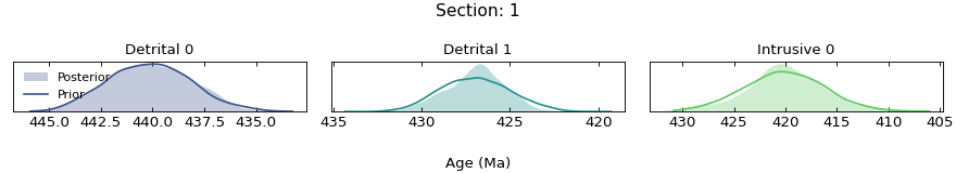

Parameters:

full_trace: arviz.InferenceData: An arviz.InferenceData object containing the full set of prior and posterior samples from get_trace() in stratmc.inference.
sample_df: pandas.DataFrame: pandas.DataFrame containing proxy data for all sections.
ages_df: pandas.DataFrame: pandas.DataFrame containing age constraints for all sections.
section: str: Name of target section.
cmap: str, optional: Name of seaborn color palette to use for age distributions. Defaults to ‘viridis’.

Returns:

fig: matplotlib.pyplot.figure: Figure with prior and posterior limiting age constraint distributions.

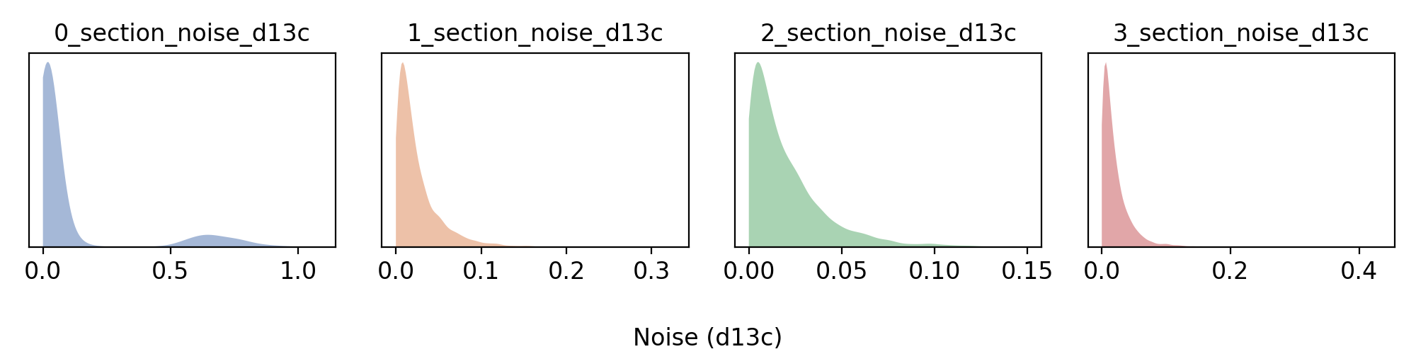
stratmc.plotting.noise_summary(full_trace, **kwargs)[source]#

Plot posterior noise distributions for each section or group of samples (depending on noise_type used in build_model()) for a given proxy. If multiple proxies were included in the inference, pass a proxy argument to specify which noise terms to plot.

(Source code, png, hires.png, pdf)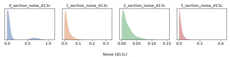

Parameters:

full_trace: arviz.InferenceData: An arviz.InferenceData object containing the full set of prior and posterior samples from get_trace in stratmc.inference.
proxy: str, optional: Target proxy; only required if more than one proxy was included in the inference.

Returns:

fig: matplotlib.pyplot.figure: Figure with noise distributions for each section or group of samples.

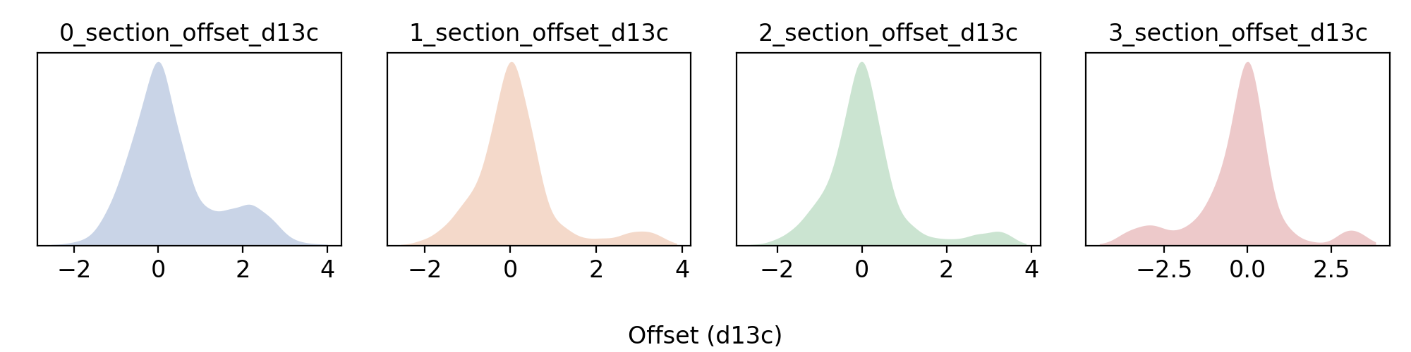
stratmc.plotting.offset_summary(full_trace, **kwargs)[source]#

Plot posterior offset distributions for each section or group of samples (depending on offset_type used in build_model()). If multiple proxies were included in the inference, pass a proxy argument to specify which offset terms to plot.

(Source code, png, hires.png, pdf)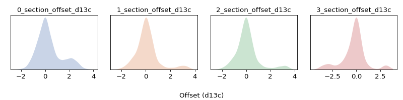

Parameters:

full_trace: arviz.InferenceData: An arviz.InferenceData object containing the full set of prior and posterior samples from get_trace() in stratmc.inference.
proxy: str, optional: Target proxy; only required if more than one proxy was included in the inference.

Returns:

fig: matplotlib.pyplot.figure: Figure with offset distributions for each section or group of samples.

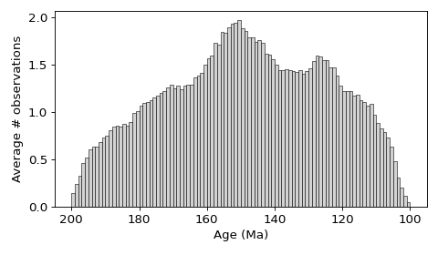
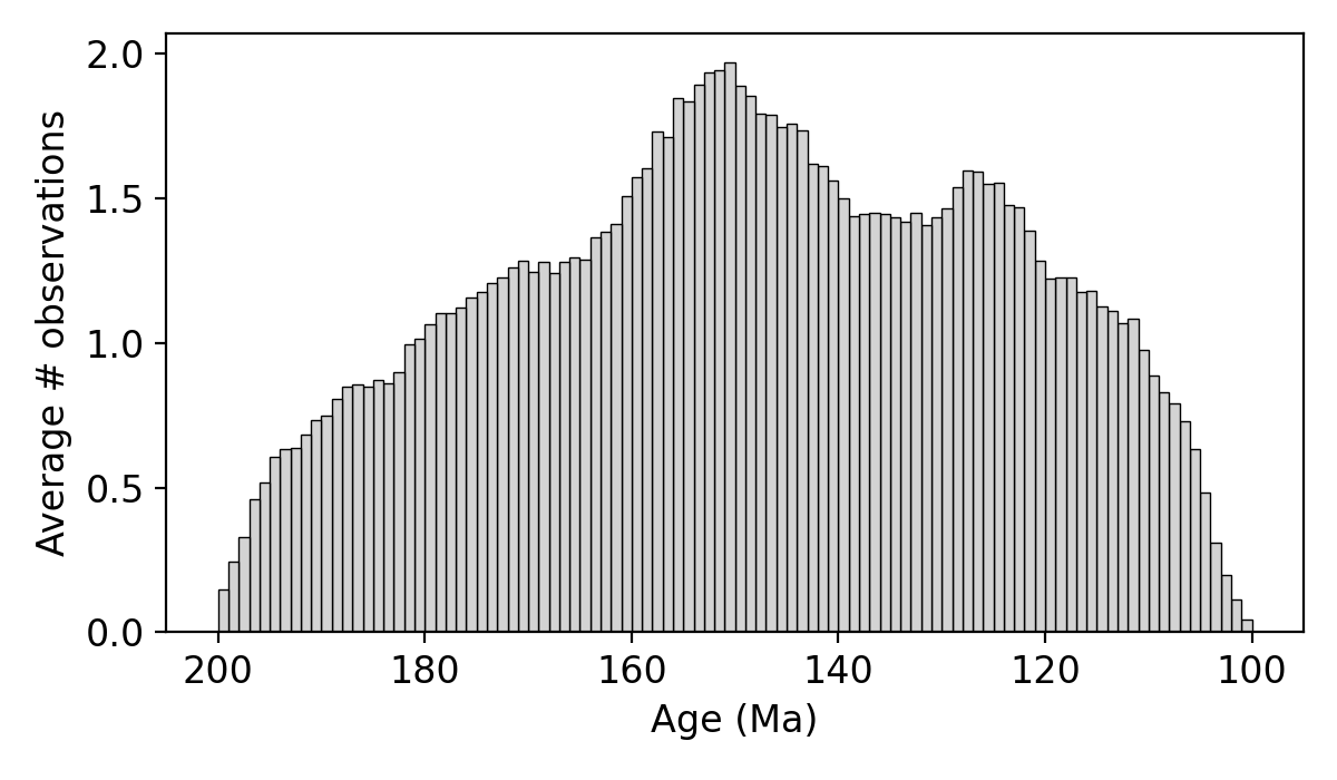
stratmc.plotting.proxy_data_density(full_trace, time_grid=None, figsize=(6, 3.5), **kwargs)[source]#

Plot the mean number proxy observations in discrete time bins (averaged over all posterior draws). This plot can be used to determine where proxy observations are relatively sparse, and additional observations may improve the inference.

(Source code, png, hires.png, pdf)

Parameters:

full_trace: arviz.InferenceData: An arviz.InferenceData object containing the full set of prior and posterior samples from get_trace() in stratmc.inference.
time_grid: np.array, optional: Time bin edges; if not provided, defaults to the ages array passed to get_trace().

Returns:

fig: matplotlib.pyplot.figure: Figure with bar plot of mean number of observations in each time bin.

stratmc.plotting.proxy_data_gaps(full_trace, time_grid=None, yaxis='percentage', figsize=(6, 3.5), **kwargs)[source]#

For a set of discrete time bins, shows the number of draws from the posterior where there are no proxy observations (i.e., where there are temporal gaps in the proxy data). This plot can be used to determine where additional observations are needed to improve the inference.

(Source code, png, hires.png, pdf)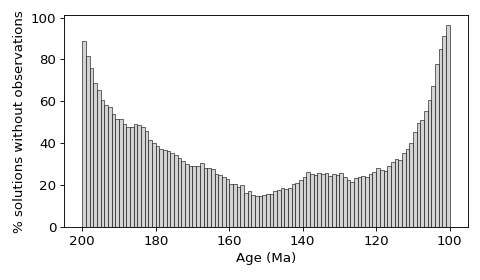

Parameters:

full_trace: arviz.InferenceData: An arviz.InferenceData object containing the full set of prior and posterior samples from get_trace() in stratmc.inference.
time_grid: np.array, optional: Time bin edges; if not provided, defaults to the ages array passed to get_trace().
yaxis: str, optional: Set y-axis to percentage of posterior draws without observations (‘percentage’) or to the number of posterior draws without observations (‘count’). Defaults to ‘percentage’.

Returns:

fig: matplotlib.pyplot.figure: Figure with bar plot of number of posterior draws with gaps for each time bin.

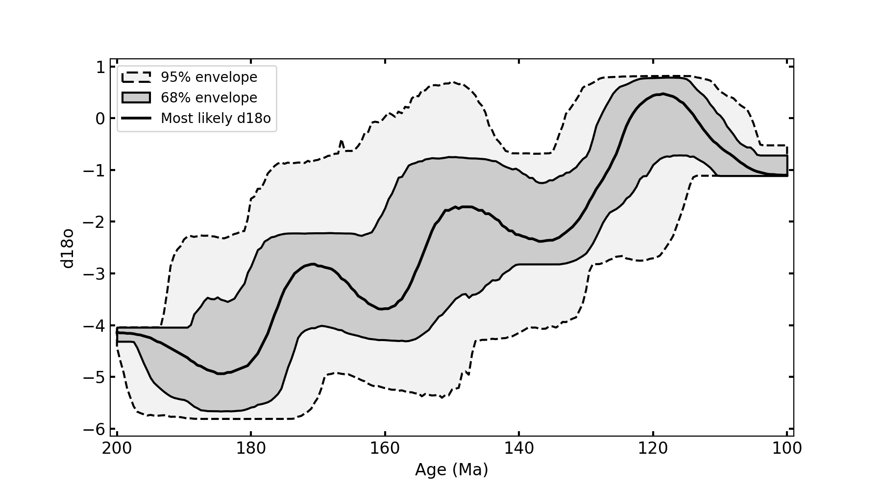
stratmc.plotting.proxy_inference(sample_df, ages_df, full_trace, legend=True, plot_constraints=False, plot_samples=False, plot_excluded_samples=False, plot_mean=False, plot_mle=False, orientation='horizontal', marker_size=20, section_legend=False, section_cmap='Spectral', **kwargs)[source]#

Plot the inferred proxy signal over time.

(Source code, png, hires.png, pdf)

Parameters:

sample_df: pandas.DataFrame: pandas.DataFrame containing proxy data for all sections.
ages_df: pandas.DataFrame: pandas.DataFrame containing age constraints for all sections.
full_trace: arviz.InferenceData: An arviz.InferenceData object containing the full set of prior and posterior samples from get_trace() in stratmc.inference.
proxy: str, optional: Tracer to plot; only required if more than one proxy was included in the inference.
legend: bool, optional: Generate a legend. Defaults to True.
plot_constraints: bool, optional: Plot age constraints for each section as dashed lines. Defaults to False.
plot_samples: bool, optional: Plot proxy observations by most likely posterior age. Defaults to False.
plot_excluded_samples: bool, optional: Plot proxy observations that were excluded from the inference (Exclude? is True in sample_df). Defaults to False.
plot_mean: bool, optional: Plot the mean as a dashed line. Defaults to False.
plot_mle: bool, optional: Plot the maximum likelihood estimate. Defaults to False.
orientation: str, optional: Orientation of figure (‘horizontal’ with age on the x-axis, or ‘vertical’ with age on the y-axis). Defaults to ‘horizontal’.
marker_size: int, optional: Size of markers if plot_samples is True. Defaults to 20.
section_legend: bool, optional: Include section names in the legend (if plot_samples is True). Defaults to False.
section_cmap: str, optional: Name of seaborn color palette to use for sections (if plot_samples is True). Defaults to ‘Spectral’.

Returns:

fig: matplotlib.pyplot.figure: Figure with the proxy signal inference.

stratmc.plotting.proxy_signal_stability(full_trace, figsize=(5, 3.5), **kwargs)[source]#

Plot the sum (over all time slices) of the residuals between the median inferred proxy signal when all N chains are considered compared to when 1 to N-1 chains are considered. When the posterior has been sufficiently explored, the residuals will stabilize and approach zero; if they have not stabilized, then additional chains should be run.

To consider chains from multiple traces associated with the same inference model, first combine the traces (saved as NetCDF files) using combine_traces() in stratmc.data.

(Source code, png, hires.png, pdf)

Parameters:

full_trace: arviz.InferenceData: An arviz.InferenceData object containing the full set of prior and posterior samples from get_trace() in stratmc.inference.
proxy: str, optional: Target proxy; only required if more than one proxy was included in the inference.

Returns:

fig: matplotlib.pyplot.figure: Figure showing the stability of the proxy signal inference.

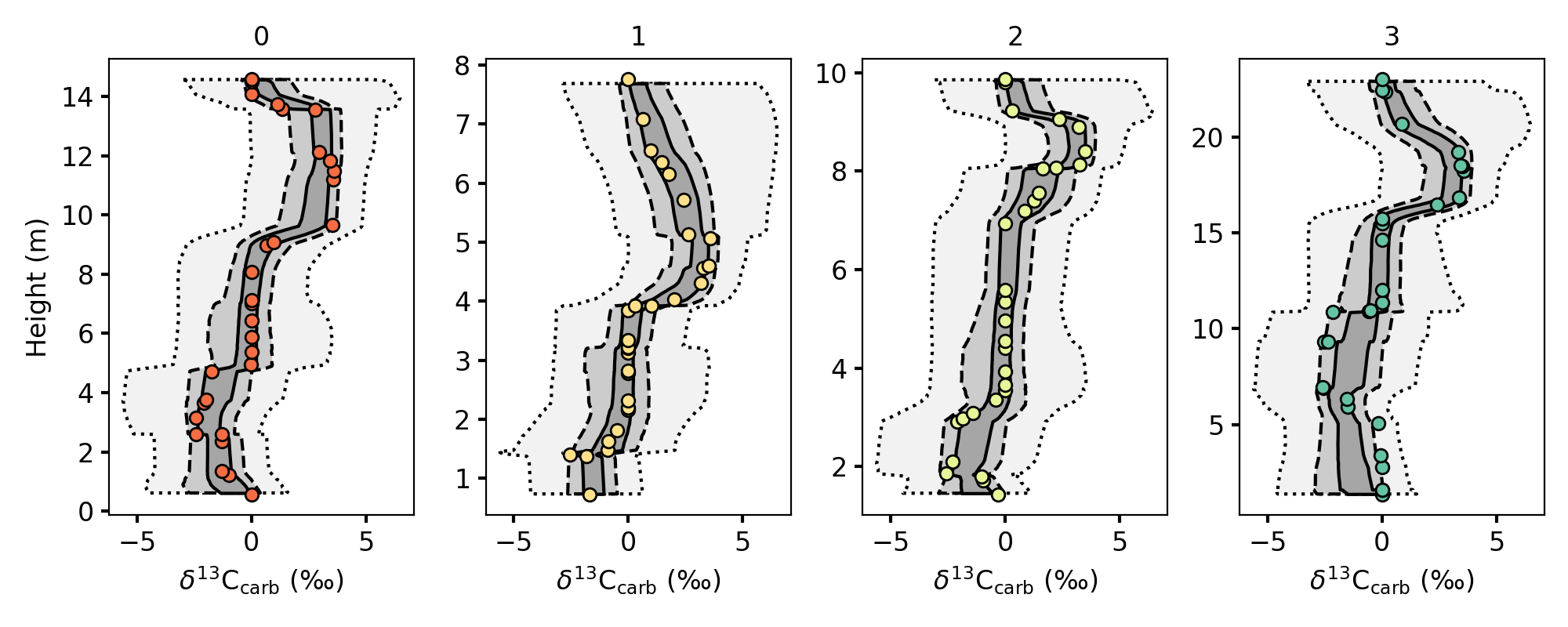
stratmc.plotting.proxy_strat(sample_df, ages_df, proxy='d13c', plot_constraints=True, plot_excluded_samples=False, cmap='Spectral', legend=False, **kwargs)[source]#

Plot stratigraphic data (proxy observations and age constraints) for each section.

(Source code)

Parameters:

sample_df: pandas.DataFrame: pandas.DataFrame containing proxy data for all sections.
ages_df: pandas.DataFrame: pandas.DataFrame containing age constraints for all sections.
proxy: str, optional: Name of proxy. Defaults to ‘d13c’.
sections: list(str) or numpy.array(str), optional: List of sections to plot. Defaults to all sections in sample_df.
plot_constraints: bool, optional: Whether to plot age constraints as dashed lines. Ages are printed above dashed lines by defalut; to turn off age labels, pass print_ages = False.
plot_excluded_samples: bool, optional: Whether to plot proxy observations for excluded samples (Exclude? is True in sample_df) as red dots. Defaults to False.
cmap: str, optional: Name of seaborn color palette to use for sections. Defaults to ‘Spectral’.
legend: bool, optional: Generate a legend. Defaults to False.
print_ages: bool, optional: Print ages as text on figure.

Returns:

fig: matplotlib.pyplot.figure: Figure with observations for each section.

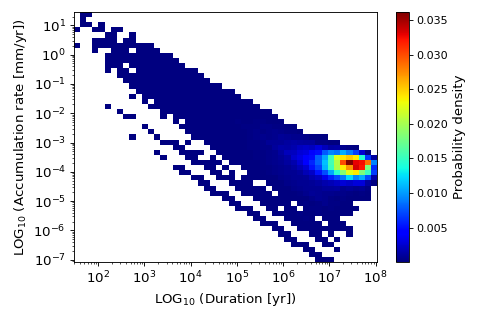
stratmc.plotting.sadler_plot(full_trace, sample_df, ages_df, method='density', duration_bins=50, rate_bins=50, scale='log', include_age_constraints=True, density_cmap='jet', section_cmap='Spectral', figsize=(6, 4), **kwargs)[source]#

Plot accumulation rate against duration.

(Source code, png, hires.png, pdf)

Parameters:

full_trace: arviz.InferenceData: An arviz.InferenceData object containing the full set of prior and posterior samples from get_trace() in stratmc.inference.
sample_df: pandas.DataFrame: pandas.DataFrame containing proxy data for all sections.
ages_df: pandas.DataFrame: pandas.DataFrame containing age constraints for all sections.
method: str, optional: Plot as a 2D histogram (‘density’) or as a scatter plot (‘scatter’). The density plot will combine data for all sections in sections, while a scatter plot will assign a unique color to each section. Defaults to ‘density’.
duration_bins: int, optional: Number of bin edges to use for the duration data. Defaults to 50.
rate_bins: int, optional: Number of bin edges to use for the rate data. Defaults to 50.
scale: str, optional: Scaling for x- and y-axes (‘linear’ or ‘log’). Defaults to ‘log’.
sections: list(str) numpy.array(str), optional: List of target sections. Defaults to all sections in sample_df.
include_age_constraints: bool, optional: Include age constraints in sedimentation rate calculations. Defaults to False.
density_cmap: str, optional: Name of matplotlib colormap to use for probability density if method is ‘density’. Defaults to ‘jet’.
section_cmap: str, optional: Name of seaborn color palette to use for sections if method is ‘scatter’. Defaults to ‘Spectral’.

Returns:

fig: matplotlib.pyplot.figure: Figure with sediment accumulation rate plotted against duration.

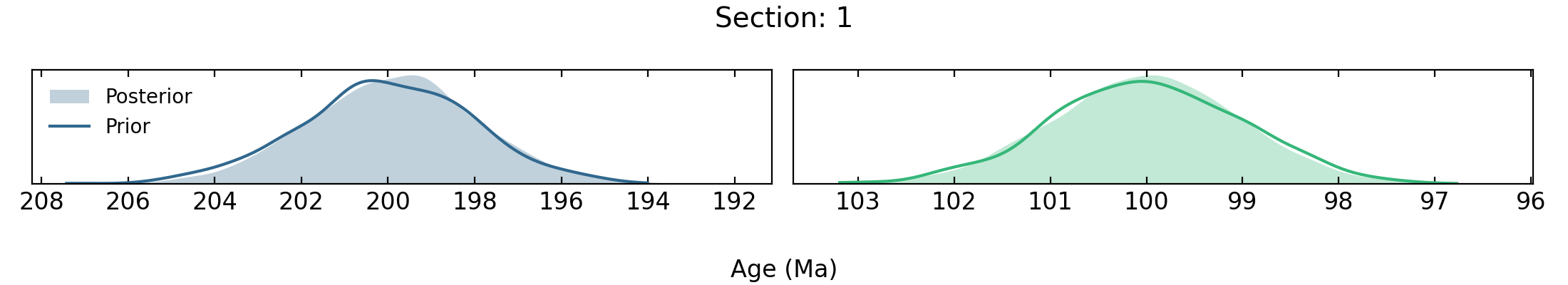
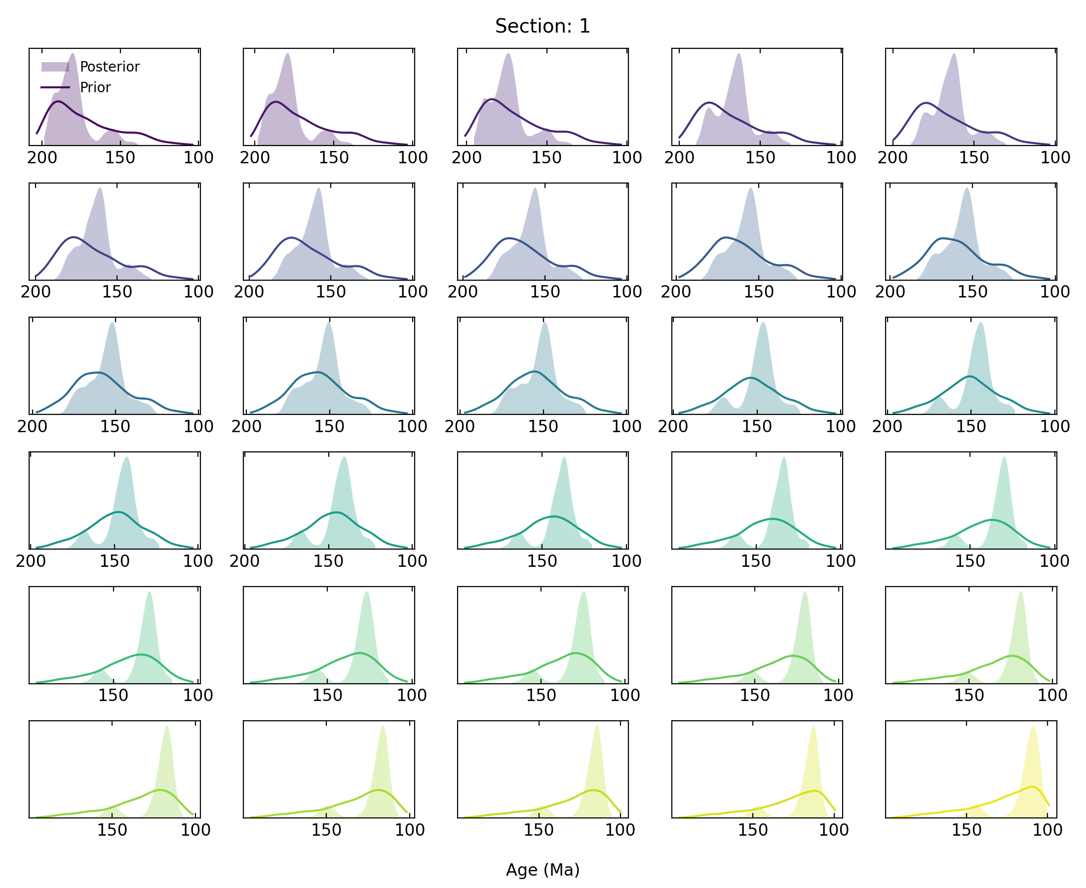
stratmc.plotting.sample_ages(full_trace, sample_df, section, plot_excluded_samples=False, plot_prior=True, cmap='viridis')[source]#

Plot sample age prior and posterior distributions for a given section. Each subplot contains posterior distributions for a different sample.

(Source code, png, hires.png, pdf)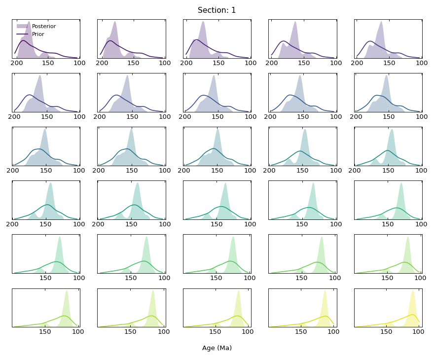

Parameters:

full_trace: arviz.InferenceData: An arviz.InferenceData object containing the full set of posterior and prior samples from get_trace() in stratmc.inference.
sample_df: pandas.DataFrame: pandas.DataFrame containing proxy data for all sections.
section: str: Name of target section.
plot_excluded_samples: bool, optional: Plot age distributions for proxy observations that were excluded from the inference (Exclude? is True in sample_df). Defaults to False.
plot_prior: bool, optional: Plot prior distributions for sample ages. Defaults to True.
cmap: str, optional: Name of seaborn color palette to use for age distributions. Defaults to ‘viridis’.

Returns:

fig: matplotlib.pyplot.figure: Figure with prior and posterior sample age distributions.

stratmc.plotting.sample_ages_per_chain(full_trace, sample_df, section, chains=None, plot_prior=False, plot_excluded_samples=False, legend=True, cmap='viridis')[source]#

Plot sample age posterior distributions for a given section, with separate distributions for each chain. Each subplot contains posterior distributions for a different sample. Use to check for posterior multimodality (in this example, each chain has explored a different mode of the posterior age distributions).

(Source code, png, hires.png, pdf)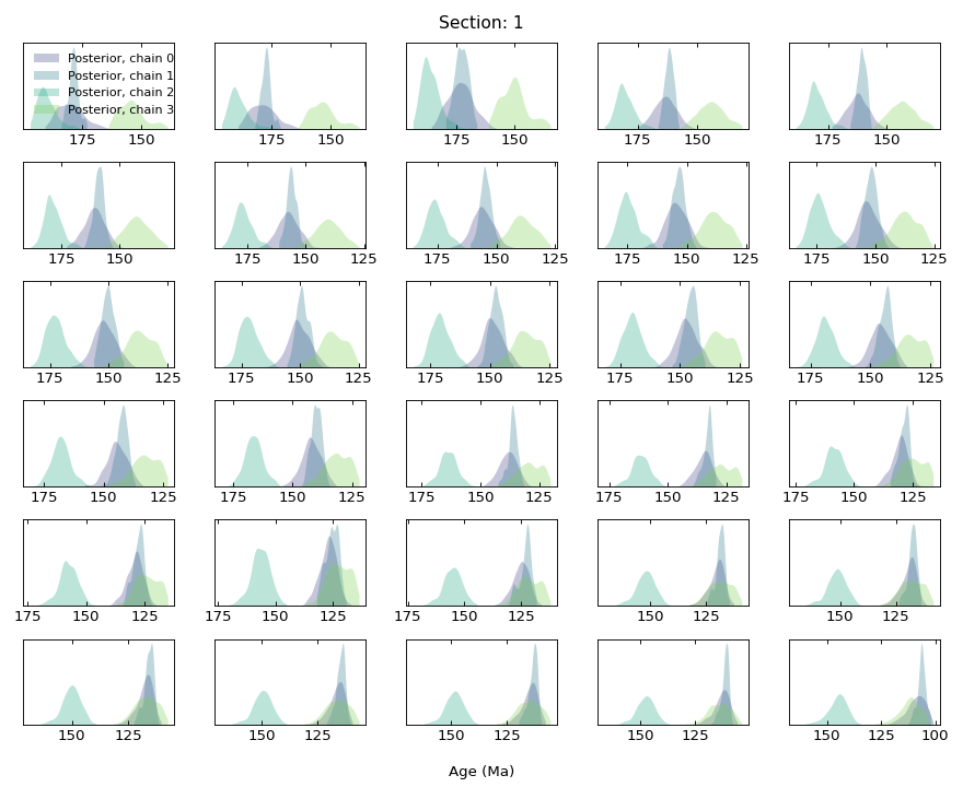

Parameters:

full_trace: arviz.InferenceData: An arviz.InferenceData object containing the full set of prior and posterior samples from get_trace() in stratmc.inference.
sample_df: pandas.DataFrame: pandas.DataFrame containing proxy data for all sections.
section: str: Name of target section.
chains: list(int) or numpy.array(int); optional: Indices of chains to include; optional (defaults to all chains).
plot_prior: bool, optional: Plot prior distributions for sample ages. Defaults to False.
plot_excluded_samples: bool, optional: Plot age distributions for proxy observations that were excluded from the inference (Exclude? is True in sample_df). Defaults to False.
legend: bool, optional: Generate a legend. Defaults to True.
cmap: str, optional: Name of seaborn color palette to use for different chains. Defaults to ‘viridis’.

Returns:

fig: matplotlib.pyplot.figure: Figure with per-chain posterior sample age distributions.

stratmc.plotting.section_age_range(full_trace, sample_df, ages_df, lower_age, upper_age, legend=True, section_cmap='Spectral', **kwargs)[source]#

Plot the stratigraphic interval corresponding to a given age range (based on the posterior section age models). If sections is not provided, includes each section that overlaps the target age range.

(Source code, png, hires.png, pdf)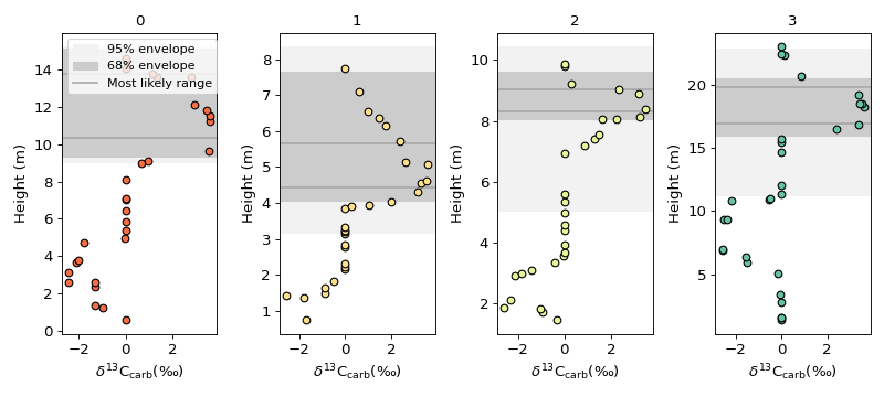

Parameters:

full_trace: arviz.InferenceData: An arviz.InferenceData object containing the full set of prior and posterior samples from get_trace() in stratmc.inference.
sample_df: pandas.DataFrame: pandas.DataFrame containing proxy data for all sections.
ages_df: pandas.DataFrame: pandas.DataFrame containing age constraints for all sections.
lower_age: float: Lower bound (youngest) of the target age interval.
upper_age: float: Upper bound (oldest) of the target age interval.
legend: bool, optional: Generate a legend. Defaults to True.
cmap: str, optional: Name of seaborn color palette to use for sections. Defaults to ‘Spectral’.

Returns:

fig: matplotlib.pyplot.figure: Tracer stratigraphy for each section, with the stratigraphic interval corresponding to the input age range highlighted.

stratmc.plotting.section_proxy_residuals(full_trace, sample_df, legend=True, cmap='Spectral', plot_mle=False, include_excluded_samples=False, **kwargs)[source]#

Plot the residuals between the observed proxy values for each section and the inferred proxy signal (using the posterior section age models to map the signal back to height in section). Use to check for stratigraphic trends in the residuals, which may give insight to the processes that cause noisy sections to deviate from the inferred common signal. If multiple proxies were included in the inference, pass a proxy argument.

(Source code, png, hires.png, pdf)

Parameters:

full_trace: arviz.InferenceData: An arviz.InferenceData object containing the full set of prior and posterior samples from get_trace() in stratmc.inference.
sample_df: pandas.DataFrame: pandas.DataFrame containing proxy data for all sections.
legend: bool, optional: Generate a legend. Defaults to True.
cmap: str, optional: Name of seaborn color palette to use for sections. Defaults to ‘Spectral’.
plot_mle: bool, optional: Plot the maximum likelihood estimate as a line. Defaults to False.
proxy: str, optional: Target proxy; only required if more than one proxy was included in the inference.
include_excluded_samples: bool, optional: Whether to plot the residuals for samples that were excluded from the inference (Exclude? is True in sample_df). Defaults to False.

Returns:

fig: matplotlib.pyplot.figure: Figure with residuals for each section.

stratmc.plotting.section_proxy_signal(full_trace, sample_df, ages_df, include_radiometric_ages=False, plot_constraints=False, plot_mle=False, yax='height', legend=False, cmap='Spectral', **kwargs)[source]#

Map the posterior proxy signal back to height in each section (using its most likely posterior age model), and plot alongside the proxy observations (plotted by most likely posterior age).

(Source code, png, hires.png, pdf)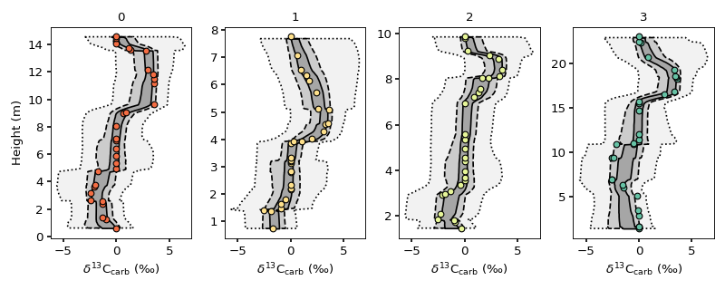

Parameters:

full_trace: arviz.InferenceData: An arviz.InferenceData object containing the full set of prior and posterior samples from get_trace() in stratmc.inference.
sample_df: pandas.DataFrame: pandas.DataFrame containing proxy data for all sections.
ages_df: pandas.DataFrame: pandas.DataFrame containing age constraints for all sections.
include_radiometric_ages: bool, optional: Whether to consider radiometric ages in the posterior age model for each section. Defaults to False.
plot_constraints: bool, optional: Plot age constraints for each section as dashed lines. Defaults to False.
plot_mle: bool, optional: Plot the maximum likelihood estimate for the proxy signal as a line. Defaults to False.
yax: str, optional: Scale for the y-axis (‘height’ or ‘age’). Defaults to ‘height’.
legend: bool, optional: Generate a legend. Defaults to True.
cmap: str, optional: Name of seaborn color palette to use for sections. Defaults to ‘Spectral’.
proxy: str, optional: Tracer to plot; only required if more than one proxy was included in the inference.

Returns:

fig: matplotlib.pyplot.figure: Figure with inferred proxy signal mapped to height in each section.

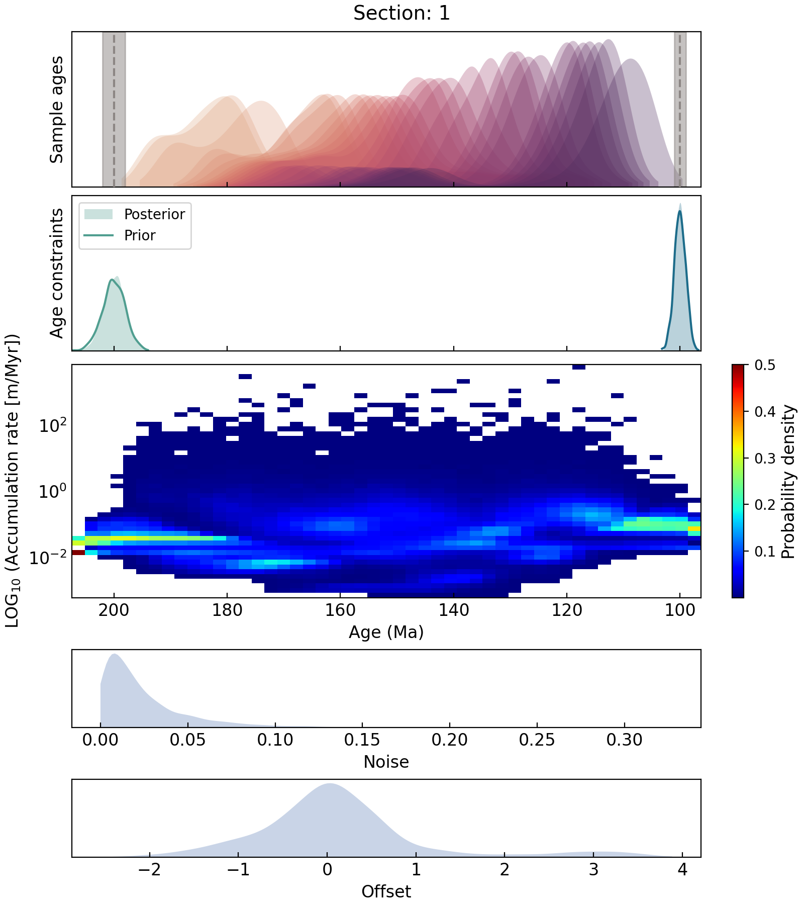
stratmc.plotting.section_summary(sample_df, ages_df, full_trace, section, plot_excluded_samples=False, plot_noise_prior=False, plot_offset_prior=False, include_age_constraints_sedrate=True, figsize=(8, 9))[source]#

For a given section, plot posterior estimates of sample age, sedimentation rate, noise, and offset. Noise and offset terms must be either per-section or global; to plot per-sample noise and offset terms, use noise_summary() and offset_summary().

(Source code, png, hires.png, pdf)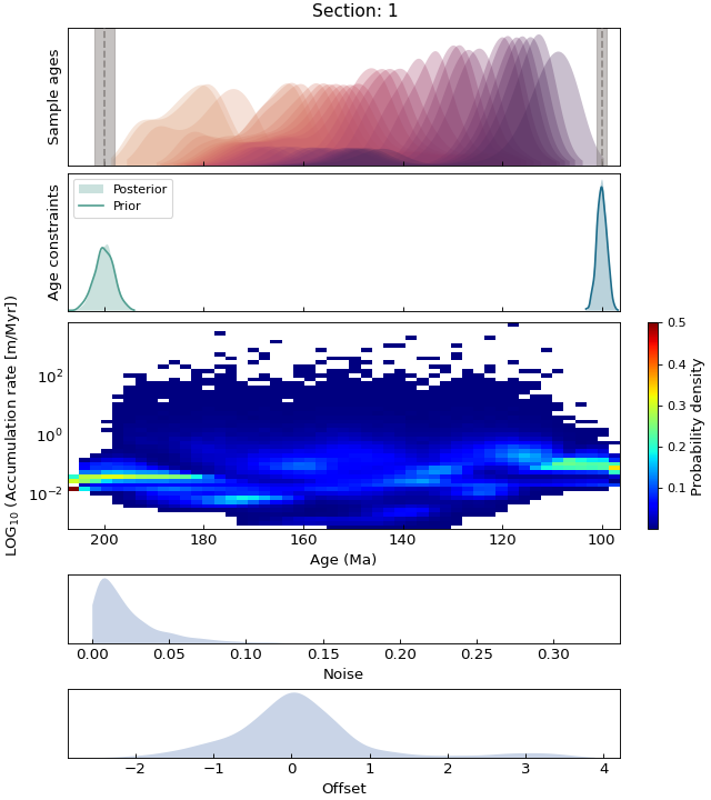

Parameters:

sample_df: pandas.DataFrame: pandas.DataFrame containing proxy data for all sections.
ages_df: pandas.DataFrame: pandas.DataFrame containing age constraints for all sections.
full_trace: arviz.InferenceData: An arviz.InferenceData object containing the full set of prior and posterior samples from get_trace() in stratmc.inference.
section: str: Name of target section.
plot_excluded_samples: bool, optional: Plot age estimates for proxy observations that were excluded from the inference (Exclude? is True in sample_df). Defaults to False.
plot_noise_prior: bool, optional: Plot prior distribution for noise term. Defaults to False.
plot_offset_prior: bool, optional: Plot prior distribution for offset term. Defaults to False.
include_age_constraints_sedrate: bool, optional: Include age constraints in sedimentation rate calculations. Defaults to True.

Returns:

fig: matplotlib.pyplot.figure: Figure summarizing posterior sample ages, sedimentation rate, and posterior noise and offset terms for the input section.

Plotting#

This Page